 WWW-POSIM v0.6.16
Physics-based sonar preview
The physics-based sonar preview simulates echoes from an underwater scene and displays their intensity by range and bearing. The images below show an exploratory experiment recorded with a dedicated sensor configuration. Reproducing it requires the matching sonar provider and sensor settings.
Runtime and sensor selection
Open Workspace → Custom robots → Build vehicle and check Forward multibeam availability. Provider required means the host needs a compatible acoustic plugin. When available, select the sensor, save its mount and rate, then start a world with that vehicle. Topics and frames follow the saved sensor manifest.
A native package can include a verified provider matched to its selected engine. If that provider is missing or fails validation, multibeam remains unavailable; vehicles that do not use it can still start. Native sonar also requires a camera in the composed scene. The installed workspace normally supplies its observer camera, so a sonar-only robot payload does not require an extra robot camera. A custom scene using native sonar with neither an observer camera nor a standard camera is rejected before Gazebo starts. Provider availability is separate from mission readiness and control validation.
A multibeam image, single Ping range, DVL velocity and SLAM map are different outputs. See Optional sensors and providers and the POSIM sonar documentation for runtime requirements. The comparison recording does not establish availability of every sonar or SLAM feature in an installed app.
Acoustic processing catalogue
- Ray geometry → range and surface normal
Gazebo samples the scene within the horizontal/vertical fan. Mount pose, angular sampling and visibility masks determine which surfaces contribute.
- Scattering → complex frequency response
The point-scattering model combines range, surface orientation, reflectivity, propagation attenuation and phase. Stochastic terms produce speckle.
- Beam correction → range transform
Beam correction mixes the frequency responses; the configured frequency window and FFT processing form range samples. Range bins must match the transform length and sound-speed/bandwidth calibration.
- Raw acoustic observation → display
Publish range/beam intensity with metadata, then apply presentation gain and fan projection. Ray-geometry points are a separate output.
| Technology | Concrete implementation | Interpretation |
|---|---|---|
| Geometry sampling | Gazebo ray rendering and the provider's spherical ray geometry; the application adapter derives surface normals from a local neighbourhood of valid points. | Scene geometry and sampling density limit features. RGB lighting is not acoustic reflectivity. |
| Point scattering | Surface reflectivity/orientation, two-way propagation attenuation and per-frequency phase contribute to a complex return. | A physically motivated approximation; it does not solve the full acoustic wave equation around the scene. |
| WGPU backscatter | Rust hosts WGSL compute kernels. Backscatter accumulation, fixed-point-to-float conversion, beam-correction matrix multiplication and FFT/readback form the GPU pipeline. | WGPU can use compatible NVIDIA or non-NVIDIA adapters. Availability and throughput depend on the actual driver, adapter and render environment. |
| Frequency/range processing | Windowing controls range sidelobes. The WGPU implementation supports exact transform lengths, including a Bluestein path for non-power-of-two sizes. | The number of displayed pixels is not independent range resolution. Preserve frequency sampling, bandwidth, sound speed and bin metadata. |
| Presentation | Display gain, colour map and range/bearing or metric-fan projection visualize the acoustic observation. | Save raw intensity as well as display settings when comparing targets; brightness alone is not calibrated target strength. |
| Geometry point cloud | Ray intersections can be bridged as PointCloud2 for geometric debugging. |
It is not a set of reconstructed acoustic detections and is not a SLAM map. |
Compute backends and parameters
The dedicated provider supports auto, wgpu, cuda and cpu. auto tries CUDA, WGPU and CPU in that order. Explicit GPU selection requires successful initialization. WGPU uses Metal on native macOS and Vulkan on Linux; CPU selects acoustic computation on the CPU. All paths still require Gazebo rendering for scene sampling. A Linux container on a Mac does not inherit native Metal access.
| Parameter | Effect and dependency |
|---|---|
| Horizontal beams, vertical rays, angular limits | Set fan coverage and angular sampling. More vertical rays sample elevation; the resulting 2D intensity image still combines elevation contributions. |
sonarFreq, bandwidth, soundSpeed |
Carrier frequency in Hz, bandwidth in Hz and assumed sound speed in m/s control the propagation/range calculation. |
Ray min/max, maxDistance |
Geometric sampling and acoustic processing range must agree. |
raySkips |
Reduces the rays used by acoustic processing, trading sampling for computation. |
sourceLevel, reflectivity, attenuation |
Set source/scene contributions to the model. They require calibration before interpreting output as a particular physical instrument. |
| Frequency window | Tapers sampled frequency content to control sidelobes; retained in the provider/application processing configuration. |
sensorGain, display mode |
Change presentation. Retain them when comparing exported images. |
update_rate, logging |
Request measurement cadence and diagnostic recording; neither guarantees achieved sensor Hz. |
frameName, topic names, visibility mask |
Define the observation frame, message routes and contributing scene geometry. |
Imaging multibeam sonar gives the application's initial fan, rate and range. Build-time backend support and runtime selection must both be recorded. The provider log reports the selected backend; a repository's existence or a GPU brand alone does not establish a working sensor.
The public provider implementation contains the C++ Gazebo sensor and Rust/WGPU library. WWW-POSIM adds model composition, provider compatibility checks and geometry/window/display adaptations. The base POSIM package and this optional provider can have different selected revisions.
Reading the observation
Raw marine_acoustic_msgs/ProjectedSonarImage carries the acoustic observation; sensor_msgs/Image is its display form. A straight wall can curve on a bearing-versus-range plot because slant range changes with bearing. A metric fan uses a different projection. Neither 2D view uniquely resolves height within the vertical fan. Mount attitude, bottom returns, surface-normal estimation and multipath-like artifacts can also affect appearance.
Keep the scene, final sensor SDF, provider/backend, acquisition time, vehicle pose, raw observation and gain/window settings together. The following controlled-removal comparison illustrates response changes; it does not establish general detection performance.
Three objects and their sonar returns
A BlueROV2 held position underwater while three physical objects were removed one at a time. The reference camera was mounted beside the sonar. The seabed and other background geometry remained in the scene.
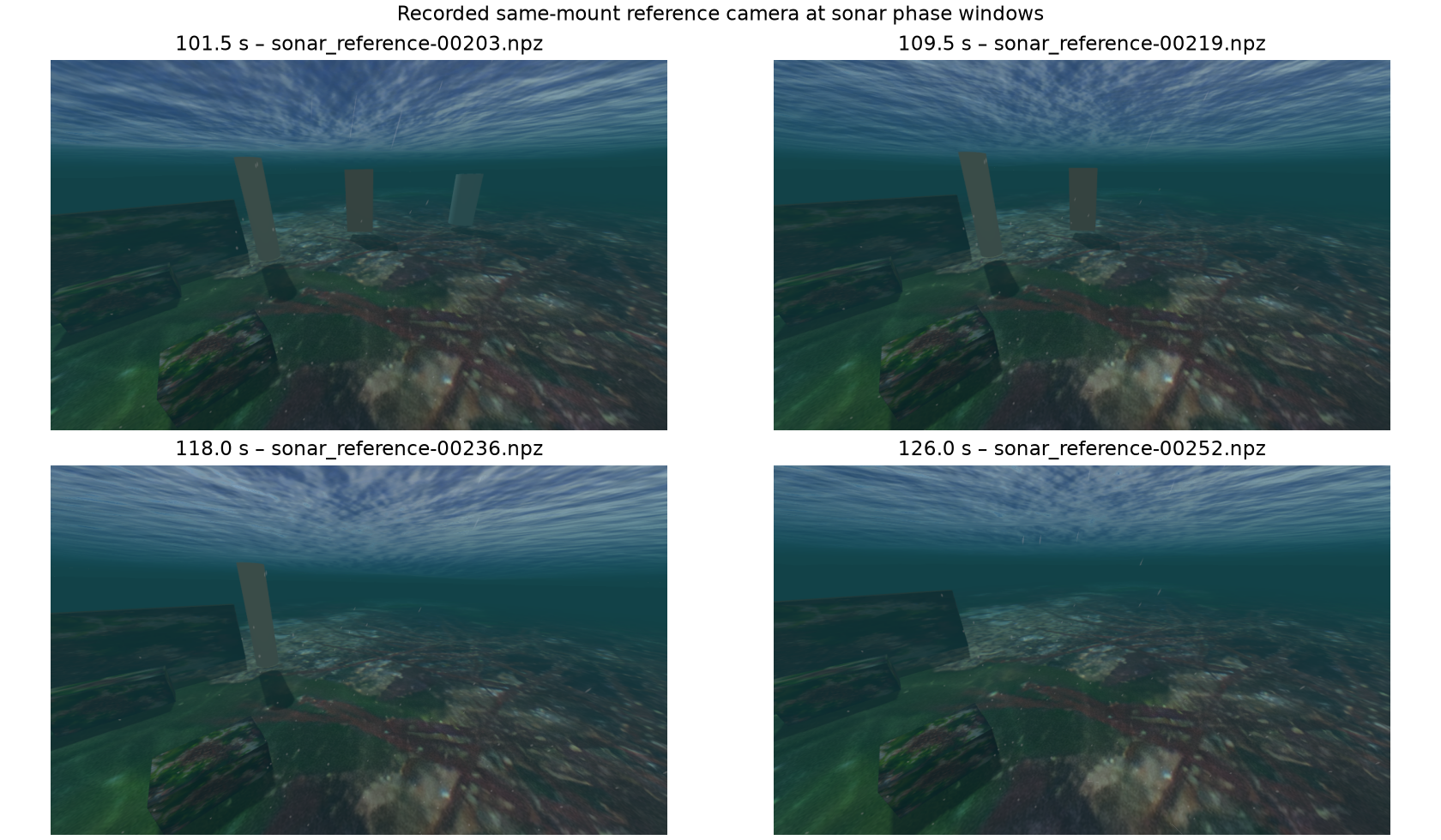
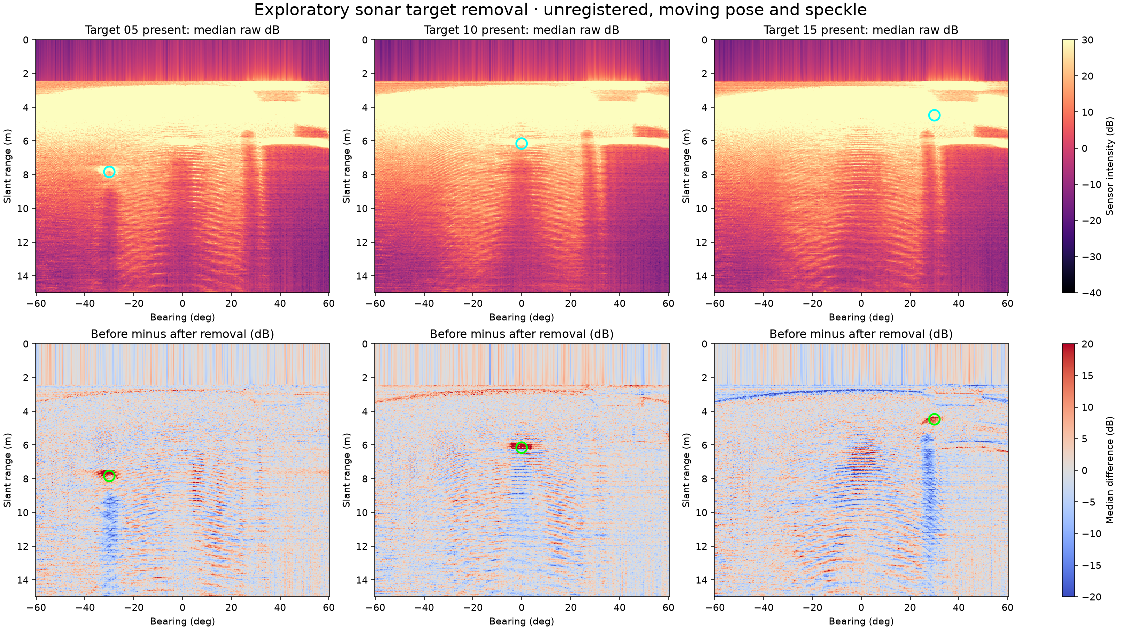
The horizontal axis is bearing in degrees; the vertical axis is slant range in metres. Warmer colours in the lower plots indicate a stronger median return before removal. Each plot uses a short window of recorded sensor frames. Changes near the nominal locations are consistent with the removals, but the seabed, pose changes, speckle and processing artifacts also affect the image. This experiment alone does not uniquely identify each return or establish detection accuracy.
The recording used a custom 60° vertical fan tilted 20° down, a 0–15 m display and disabled surface reflections. These settings were chosen for the experiment and differ from the usual sensor configuration. The vehicle held position, but moved slightly; the comparison was not registered to a fixed pose.