 WWW-POSIM v0.6.16
Terrain generation algorithms
Numeric elevation and depth define the terrain. OSM defines the coastline mask, and Sentinel-2 supplies land colour.
Processing flow
- 1. Region → metric grid
Convert the requested WGS84 centre to a local AEQD frame. Sample an N × N grid with x east, y north and z up; interval = field width / (N − 1).
- 2. Sample elevation and depth
Interpolate GEBCO as the baseline and GLO-30 for land. Select valid regional depth per water vertex; configured Cesium numeric exports have priority, then available sources by native spacing.
- 3. Extract OSM land polygons
Read the OSM-derived land shapefile, check EPSG:4326 and clip intersecting polygons to 0.05° atlas cells. Union the polygons and save land.json. The coastline is not extracted from satellite colours.
- 4. Prepare a verified satellite atlas
Query recent Sentinel-2 L2A scenes through STAC. Check RGB coverage and the scene classification layer; accept at most 5% locally invalid pixels, including clouds and shadows. Record acquisition time and hashes.
- 5. Apply the coastline to the numeric field
Use Shapely point-in-polygon tests at mesh vertices. Mapped land uses finite GLO-30 heights; water retains supported numeric depth. Coastal interpolation requires nearby measured ocean samples. Reject an incomplete candidate and record the fallback.
- 6. Build collision and visual meshes
Triangulate the numeric lattice for collisions. Build full and reduced visual meshes for streaming tiles, retaining boundary and shoreline-transition samples. Project land imagery onto UV coordinates and apply repeating sand to the seabed. Animated water is separate.
- 7. Validate → save → ready
Export SDF, meshes, numeric arrays and provenance; run gz sdf -k. Automatic land fields wait for verified imagery before publication. Store completed assets in the cache; report failures or cancel and clean up the job.
- 8. Move → select LOD → verify coverage
In on-demand worlds, choose visual detail from the vehicle's current tile, prepare approaching tiles and verify collision coverage. Change visual entities without replacing their full collision meshes. Reuse cached geometry when returning.
Terrain LOD: detail near the vehicle
LOD (level of detail) reduces the geometry drawn for distant terrain. In an on-demand world, the vehicle's tile determines the level; zooming the scene camera does not change this rule. It applies to land and seabed.
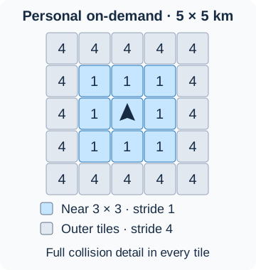
| Stage | Input → method → result |
|---|---|
| Near visuals | The central 3 × 3 tiles use stride 1: every numeric grid vertex is drawn. |
| Distant visuals | Outside that square, stride 4 selects every fourth interior sample in each direction. All tile-edge samples and cells crossing the shallow/coast material transition remain. Delaunay triangulation joins the retained vertices. The result is not a uniform 33 × 33 mesh or an exact sixteen-fold triangle reduction. |
| Textures | Distant land and shallow-water textures are reduced to one-quarter width and height, with a 32-pixel minimum. Tiles share a repeating seabed texture. |
| Movement | Entering another tile changes the near square. Approaching tiles gain full visual detail; receding tiles use reduced detail while resident. |
| Physics and routing | Full numeric samples and collision meshes stay unchanged at both visual levels. Border samples are shared to avoid gaps between levels. |
Gazebo cameras and sensors that render scene geometry observe the selected visual mesh. Full collision resolution therefore does not imply identical distant camera or rendered range images at both levels. For nearby inspection, keep the target in the full-detail neighbourhood and check the actual sensor output.
A visual replacement keeps the previous native visual until the candidate is observed. If confirmation times out while a fresh native pose still confirms the previous visual, that tile keeps its current level and retries the quality change after 30 seconds. Failed candidates are removed and their absence confirmed before another candidate is created. A cleanup failure remains an error.
For a new tile, the collision instance is created once. Visual confirmation can retry up to three times. The tile is admitted only after visual, depth and contact checks pass; missing coverage still holds the vehicle. Visual retries do not lower collision resolution or mark unverified terrain ready.
Which terrain mode uses which detail?
| Mode | Numeric terrain and visual policy |
|---|---|
| Fixed custom field | Default 1 × 1 km, 513 × 513 samples, about 1.95 m spacing. Its fixed mesh does not switch to moving tile LOD. |
| Prepared KMOU / New York / Hong Kong | The centre keeps its 513 × 513 grid: KMOU is 1 × 1 km; New York and Hong Kong are 2 × 2 km. Their 6 × 6 km surroundings use a separate measured grid, full-resolution collision meshes and fixed reduced outer visuals. KMOU also has a centre collar. These packaged surroundings do not gain moving-tile detail as the vehicle approaches. |
| Personal on-demand world | 1 km tiles, 129 × 129 samples, 7.8125 m spacing. Required coverage is 5 × 5 tiles; near 3 × 3 visuals use stride 1 and the outer ring uses stride 4. |
| Public LIVE voyage | Required coverage is 7 × 7 tiles, with the same near 3 × 3 full-detail rule. Recently visited and prefetched tiles can extend the resident area. |
See On-demand terrain for generation and recovery, and Terrain, water and nearby traffic for its residency limits. LOD selection is automatic; the interface has no manual LOD slider.
Geospatial technology catalogue
| Technology | Inputs and operation | Output / interpretation |
|---|---|---|
| Local metric projection | PyProj transforms WGS 84 longitude/latitude to a region-centred azimuthal equidistant projection; longitude is always the first axis. Floating-origin transforms additionally align active runtime coordinates. | Metre-valued x/y grids with a recorded geographic datum. Local projected coordinates are not interchangeable with latitude/longitude or an FCU origin. |
| Raster sampling | GEBCO windows and land elevation are sampled on the requested grid using SciPy interpolators; raster metadata controls axes and NoData handling. | Numeric elevation, distinct from the spacing and accuracy of the original measurements. |
| Regional source selection | Configured licensed Cesium numeric data has priority. Remaining regional providers are ordered by their reported native spacing and accepted per valid marine vertex. | Per-vertex provider IDs and source records; unavailable coverage falls back through the configured policy. An imagery credential alone is not a numeric bathymetry source. |
| Coastal bathymetry support | Known water cells that coarse sampling turns into land are reconstructed from actual nearby marine samples using LinearNDInterpolator and a cKDTree support check. Nearest marine fallback is bounded to 1.5 km. |
A source-supported coastal correction; it does not invent a constant safe depth. KHOA interpolation has its own tighter 225 m support rule. |
| Land mask | Shapely polygon union and point-in-polygon tests use OSM coastline geometry, combined with finite land elevations. | Explicit land/water classification. Satellite colour does not decide whether a location is navigable water. |
| Imagery | STAC selection, scene classification, Rasterio reprojection and separate imagery quality tests prepare land textures. Numeric height and visual colour remain independent. | RGB assets with acquisition/source metadata. Prepared Hong Kong uses its attributed aerial imagery. |
| Geometry | Triangulated numeric grids form collision terrain; material masks separate land, shallow water and seabed visuals. Runtime visual LOD preserves edges and coastal transition samples. | SDF, mesh and texture assets, with a full-resolution collision path and a separate rendering budget. |
Source downloads and cache checks
Matching regional coastal cells are checked for freshness and checksum before reuse. A complete cache hit returns before preparing the global coastline archive. Missing or invalid cells follow the source refresh path.
GEBCO subset lookup uses a SQLite metadata index. Changed file sizes or modification times refresh its entries; selected candidates are checked again for source URL, raw SHA-256 and coordinate axes. An unavailable index falls back to the verified cache scan.
Regional downloads first go to a temporary file. When HTTP Content-Length is supplied, the received byte count must match it. KHOA NetCDF files must expose exactly the three variables Lat, Lon and MSL, with nonempty arrays and readable final elements. The file is moved into the persistent cache after validation. A rejected existing file remains available for diagnosis.
- KHOA BADA2024 file limit: 400 MiB.
- Download budget: 180 s, checked before and after incremental reads of up to 256 KiB.
- Socket idle timeout: 20 s. A stalled read or header wait can continue until that timeout; the download budget is not a strict total wall-clock limit.
Terrain readiness checks
WWW-POSIM checks each streamed tile with a downward RGBD camera and a temporary physical sphere. The camera measures the rendered surface depth. Gazebo drops the sphere onto the collision mesh; fresh pose readings confirm contact before the tile counts as usable coverage.
- Probe: radius 0.25 m, mass 10 kg, placed 1 m above the sampled surface and removed after the check.
- Contact: measure the signed shortest distance from the sphere centre to nearby mesh triangles, including their edges. This distance accounts for sloping terrain.
- Acceptance: at least eight distinct pose readings, with the latest five at 0.1–0.6 m from the surface. A recorded penetration deeper than 0.15 m, missing contact, stale poses or failed probe removal rejects the tile.
- Scope: this checks loading and contact at one local point. It does not certify every triangle, source elevation accuracy or an entire navigation route. Route clearance checks remain separate.
Artifacts and reproducibility
| Artifact | Research use |
|---|---|
projected.npz and grid metadata |
Inspect x/y/elevation arrays in the generating datum; compare paths and measurements against numeric terrain. |
manifest.json, source/provider records |
Preserve requested bounds, sample count, source choices, hashes and compatible engine/library identity. A cache hit is meaningful only for that identity. |
| Model/world SDF and collision meshes | Establish the actual contact surface and scene assembly; screenshots cannot substitute for these. |
| Visual meshes, textures and LOD metadata | Reproduce rendering and rendering-based sensor observations separately from collision accuracy. |
Tile generation, prefetching, residency and visual replacement are WWW-POSIM orchestration around POSIM-Terrain outputs. Confirmed collision coverage is required before a path enters a new area. A prepared asset, loaded collision tile and current visual image are separate readiness states.
Implementation: POSIM-Terrain at the selected source, especially terrain.py, terrain_sources.py, bathymetry.py, coastal_detail.py and floating_origin.py.
Interpretation
Source measurement resolution, generated grid spacing, visual LOD and image resolution describe different things. A finer mesh or texture cannot add measurements missing from the original dataset; narrow coastal features can be missed. All-water fields can finish without land imagery. A camera close-up over water can hide the coast: zoom out in World view or inspect Map before concluding that terrain is missing.
Related documentation and implementation
Generate terrain for your site · Route planning & control · Simulation, rendering & sensors
POSIM-Terrain implementation: terrain.py, terrain_sources.py, bathymetry.py, coastal_detail.py, seabed_visual.py. Packaged results use the application-selected library revision; inspect manifest.json and source-providers.json for actual sources and assumptions.
Terrain sources and readiness
Prepared fields have 513 × 513 terrain samples. KMOU covers 1 × 1 km; New York and Hong Kong each cover 2 × 2 km (about 3.91 m between terrain samples).
| Prepared field | Centre (latitude, longitude) | Imagery |
|---|---|---|
| KMOU waterfront | 35.077175, 129.085815 | Sentinel-2 |
| New York harbour | 40.70044, −74.004885 | NYC OTI aerial imagery, 2024 |
| Hong Kong harbour | 22.2899, 114.168169 | Lands Department aerial imagery, October 2018 / January 2019 |
Each prepared field includes a 6 × 6 km area arranged as 3 × 3 two-kilometre tiles. KMOU includes a collar around its 1 km centre. Surrounding tiles use lower visual resolution and measured elevation/depth sources. The WAM-V demo uses the same Hong Kong harbour terrain and satellite imagery as the prepared field.
New York and Hong Kong use 4096 × 4096 centre textures, sampled at about 49 cm per pixel. Native photographs have 6-inch and 20 cm resolution respectively. Texture detail does not increase elevation or depth accuracy. These textures are included in the bundle; automatic generation uses Sentinel-2.
NYC imagery is CC BY 4.0, NYC OTI. Hong Kong imagery is from the HKSAR Government Lands Department / CSDI Portal, tile T11-SW-B, released in 2023. Both images are cropped, reprojected and resampled. Source notices accompany each world download.
Automatic geographic worlds with land wait for verified satellite imagery before becoming ready. If imagery cannot be prepared, generation reports an error; retry after restoring source access. A saved world missing imagery needs regeneration. Satellite colour is shared by Browser and Gazebo; it does not change collision heights. The challenge preset uses an authored flat arena. To view your generated terrain, select it in the saved-world list and start that world.
Downloads show the current file, downloaded and total size, percentage, and transfer speed. When the provider does not report a total size, the progress shows the received size and speed. Select Stop to cancel the job and its download worker. Completed source files remain available for another attempt.
As automatic streaming terrain expands, missing land imagery is retried in the background. Verified imagery appears automatically while the sampled elevation and collision surface stay unchanged.
Readiness, cancellation and retry
Prepared fields remain Downloaded · Ready to use after download. Ready describes the terrain assets; after starting a world, also check fresh vehicle position and sensor reception. If files are missing or the runtime is incompatible, follow the displayed download or regeneration instructions.
Use Stop in the installed app's progress area, or Cancel during web terrain preparation. Wait for cancellation to finish before retrying. A preparing terrain, an available server slot and a running world are separate states.
If terrain is ready but land is out of view, zoom out in World or inspect Map. Check Scene → Display → Seafloor and the map overlay. See Terrain LOD: detail near the vehicle for distant detail and fixed/on-demand differences.
Geographic dataset selection
For processing order, coastline extraction, interpolation, source selection and output files, see Terrain generation algorithms.
The installed app opens with a choice: start a WAM-V or BlueROV2 demo or create your own terrain. A simulation starts after you choose it. During terrain generation or simulation startup, select Stop in the progress area to cancel the operation. Wait for cleanup to finish before starting another world.
Data selection
Configured, licensed Cesium World Bathymetry takes priority. Regional sources depend on coverage; GEBCO supplies the global fallback.
| Source | Role |
|---|---|
| Cesium World Bathymetry | Preferred when licensed numeric access is configured |
| Copernicus Marine coastal bathymetry | Regional high-resolution depth |
| EMODnet | Regional depth, primarily European waters |
| KHOA | Optional depth near Korea |
| GEBCO | Global elevation and depth fallback |
| Copernicus GLO-30 | Coastal land elevation |
| OpenStreetMap coastline | Refines land/water boundaries on the numeric grid |
| Sentinel-2 RGB | Land satellite colour |
Check access and coverage with Cesium, Copernicus Marine, EMODnet and GEBCO. Collision terrain uses numeric elevation/depth. The interface identifies the source used.
Resolution and lines
Validated OSM coastline and clear Sentinel-2 imagery enable coastal refinement. Land uses GLO-30; water uses supported numeric depth. Corrected elevations feed visuals, collision, sensors and route checks.
- New on-demand region and tiles: 1 × 1 km, 129 × 129 samples, 7.8125 m grid spacing
- Resident area: 5 × 5 tiles, covering 5 × 5 km; tile size is fixed
- Visual detail: automatic vehicle-centred Terrain LOD: detail near the vehicle, retaining edge and coastal samples
- Collision grids: full resolution in every resident tile, including offshore
- Land imagery: allocated only on tiles with land; all tiles share the repeating seabed texture
- Satellite imagery: nominal 10 m
- Unknown depth: excluded from routes
- Missing or invalid refinement: GEBCO, Copernicus and regional depth sources
- Additional downloads: background preparation
A finer mesh does not make the source measurements more accurate. Check the original sample spacing and data source against your experiment's depth requirements.
Imagery can apply independently of coastline refinement. Starting a saved region checks available imagery. The installed app retains complete source caches in the project's data/providers folder.
- World / Vehicle, Gazebo Map and sensor images: land satellite colour and sand seabed texture
- Browser Map: an optional OpenFreeMap overlay; turn off Map overlay to see the terrain's satellite colour
- Minimap: OpenFreeMap
- Seabed grid/contours: optional live overlays for visual scale and shape; off by default
- Blue/cyan imagery pixels on exposed land: green tint preserving luminance
The terrain texture blends with dark blue-grey near mean sea level. The blend is strongest at sea level and fades at both limits.
- Blend range: −1.0 to +0.5 m relative to mean sea level
Imagery and lines supply visual appearance. Elevation data determines depth and collision geometry.
On-demand terrain
The initial generated region is 1 × 1 km. The runtime also prepares neighbouring tiles for safe coverage; the loaded neighbourhood can be larger than this initial region. Fixed fields retain their separate 513 × 513 default.
Nearby terrain tiles load in the background, and recently used tiles remain available for return travel. The engine adds and removes tiles in sequence. In personal sessions, control commands pause before the robot enters an area without verified collision or sensor coverage.
Missing tiles are requested again. Adjacent tiles share border samples, and re-entry loads saved geometry.
The world voyage follows ports in itinerary order and favours coastal routes with checked depth and hull clearance. See LIVE world voyage for coastal distances and minimum depths.
Seabed texture and measurement lines
The seabed shows sand detail by default, with grid lines and contours off. Change these settings live in Scene → Scene renderer → Underwater appearance. Changes apply to the Gazebo scene and camera color feeds.
The packaged sand uses Aerial Beach 01 by Rob Tuytel, licensed CC0, with 2K color, normal and roughness maps repeating every 30 m. It represents generic sand and works offline. Terrain elevation data determines the actual geometry and depth.
Generate a seabed material atlas
Download the generator and materials ZIP, then extract it. The Python script is also available separately. Use Python 3.10 or newer with NumPy and Pillow. Run the commands from the extracted folder.
python -m pip install numpy pillow
python generate_seabed_materials.py --materials materials --output output --bounds -3000 -3000 3000 3000 --seed 321 --region-m 240 --detail-m 4 --size 1024 --green-zones materials/kmou-green-zones.json
The generator blends eight supplied materials in world coordinates: red vegetation, dense red and green vegetation, blue seabed, and mixed, white and black rocks. A shared seed keeps the distribution consistent across independently generated neighbouring areas. These are synthetic colour textures; they do not add plant height, rock geometry, collision or measured bathymetry.
This example covers 6 × 6 km at 1024 × 1024 pixels, about 5.86 m per pixel. It is an overview: small vegetation and stones are not resolved at this scale. Bounds are local east/north metres, not latitude/longitude. The top image row corresponds to maximum northing.
The new output folder contains albedo.png and manifest.json with bounds, settings and hashes. Existing output folders are rejected. Use --tile-m to split the area; --size then applies to each tile. The default budget is 67,108,864 pixels across all tiles. Reduce the extent or resolution if it is exceeded, or explicitly set --max-total-pixels after checking memory and storage. An INCOMPLETE.txt file marks failed output.
The additional dark marine-green material is concentrated around the three KMOU wreck footprints when --green-zones materials/kmou-green-zones.json is supplied. The JSON defines local x/y, core_m, fade_m and strength for each zone. Without this option, the standalone generator does not infer wreck positions. Broad dominant regions use --region-m 240; transitions blend neighbouring materials rather than applying a fine colour mosaic. Keep the generator version, input hashes and seed together when reproducing an atlas.
Green-dominant surroundings are a visual design for studying difficult RGB recognition. They do not establish sonar performance: object geometry and sonar settings remain separate, and comparison requires actual camera and sonar observations.
